In order to simplify marking the positive images, instead of marking and identifying thousands of images we decided to try marking one image and rotating the image 1 degree for a complete 360 degree rotation. We are hoping that this will still bring about enough variance in our data sets, while still increasing the hit rate without the initial overhead and pain of individually marking all images.
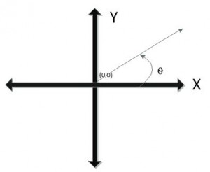
For image processing we are dealing with a left-handed coordinate system as opposed to the usual right-handed Cartesian coordinate system (typically seen in mathematics) that we usually deal with. For example, the right handed has center point (0,0) set in the middle of the graph with positive x moving right along the axis, while positive y moves up the axis.
The angle of rotation is as a counter-clockwise rotation. With this system there are negative coordinates available for plotting, where as negative values do not make sense in the context of computer graphics for positions of pixels.
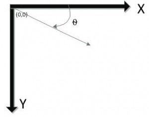
So for the left-handed Cartesian coordinate system as dealt with in computer graphics; begins with the point (0,0) in the upper left corner and positive x moving right along the axis, while positive y moves down the axis. The angle of rotation is as a clockwise rotation. So the rotation matrix would reflect the rotation difference by a -Θ(-angle) since the direction of vector rotation is counterclockwise if Θ is positive (e.g. 45°), and clockwise if Θ is negative (e.g. -45°).
Apply the rotation matrix to the following matrix multiplication table which will rotate the column vectors of the image. So the coordinates (x’,y’) of the point (x,y) after rotation are derived from the following formula.


Below is a code excerpt for getting the new new point after rotation.
//Get the distance from the center to our point of interest
int a = x - src_center.x;
int b = y - src_center.y;
double distance = sqrt((double)((a*a) + (b*b)));

//Convert the angle to radians
double radians = angle * (PI/180);

float deltaX = cos(radians) * a + sin(radians) * b;
float deltaY = cos(radians) * b - sin(radians) * a;

//Add the delta (change) values to our initial point value to get the shift and new coordinates
float newXPos = src_center.x + deltaX;
float newYPos = src_center.y + deltaY;
Tags: image processing, opencv
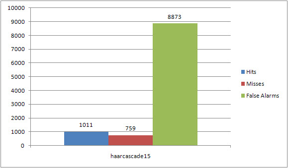
So now that the limitation of the performance application has been identified what does that mean for the previous haar classifiers we have tested and analyzed this far? Well to put it bluntly they were wrong. The results did not truly reflect the classifiers accuracy. So I took the haarcascade15, since this classifier had the best overall results without taking into account the size and position differences.
Hit rate ≈ 57.1%
The coding excerpt that handles the size and position difference values and calculates whether the detected area is considered a true positive detection (HIT).
det is a pointer to an ObjectPos struct that contains the values for the detected rectangle.ref is a pointer to an ObjectPos struct that contains the values for the referenced rectangle that was identified through the ObjectMarker.
                    found = 0;
                    for( j = 0; j < refcount; j++ )
                    {
                        distance = sqrtf( (det[i].x - ref[j].x) * (det[i].x - ref[j].x) +
                                          (det[i].y - ref[j].y) * (det[i].y - ref[j].y) );
                        if( (distance < ref[j].width * maxPosDiff) &&
                            (det[i].width > ref[j].width / maxSizeDiff) &&
                            (det[i].width < ref[j].width * maxSizeDiff) )
                        {
                            ref[j].found = 1;
                            ref[j].neghbors = MAX( ref[j].neghbors, det[i].neghbors );
                            found = 1;
                        }
                    }
With specifying the values for a size and position difference it was pretty much trial and error to see which values gave the most desirable results. These values seemed to do well, and keep the detections within bounds of the real detections.
Performance.exe -data "F:\Thesis_Research\AutomatedDetector\HaarClassifier\haarcascade15\haarcascade15.xml" -info "F:\Thesis_Research\AutomatedDetector\Test_Sets\Positive_Solar_Cavities\positivesoutput.txt" -maxSizeDiff 5 -maxPosDiff 4
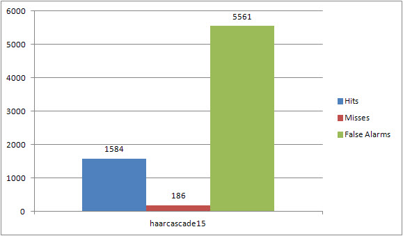
Below is the more accurate portrayal of the classifiers detection rates, this rate is about 89.5% which is definitely alot better than the 57.1% I was racking my brain over before.
Hit rate ≈ 89.4%
Tags: opencv, performance, testing outcomes, thesis, trials
When creating a classifier to use for detection of solar cavities, the steps taken are essentially creating the samples to train with, train, and then test the performance. In testing the performance, I began looking through the output, and noticed some oddity. For some of the images the performance output would classify a MISS, so I decided to do some comparison of those results by looking at the images and do a visual inspection of the performance classification results and the actual classification results. I was getting misses based on the size difference of my marked image (what I denoted as the bounds or area of the positive object) versus the classifiers size and position of what it calculates as the positive object.
Below is an excerpt from the performance output originally and for this specific image the output shows that there were no HITS and 1 MISS.
+================================+======+======+======+
|            File Name           | Hits |Missed| False|
+================================+======+======+======+
[...]
+--------------------------------+------+------+------+
|   20101231_231508_1024_0193.jpg|     0|     1|     9|
+--------------------------------+------+------+------+
But this below excerpt is when the performance tool is run specifying to not be so strict on the size and position difference when comparing that positive classification with the marked image. Now we get the HIT with no MISSES.
+================================+======+======+======+ | File Name | Hits |Missed| False| +================================+======+======+======+ [...] +--------------------------------+------+------+------+ | 20101231_231508_1024_0193.jpg| 1| 0| 7| +--------------------------------+------+------+------+Here is an example of the output image, I changed some colors to highlight which one is which. The GREEN rectangle shows essentially the marked image, while the BLUE rectangles are the classifiers detections. You can notice that the BLUE and GREEN area are not exact, but the area that the BLUE rectangle covers does still in fact include the cavity so it should have really been a positive HIT from the beginning.
So what does all this mean?
Pretty simply put, the performance values initially obtained did not truly reflect the performance of the classifier.
Tags: opencv, performance, testing outcomes, thesis
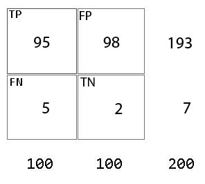
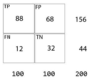
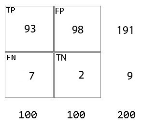
In an attempt to analyze some data as well as performance of my classifier and implementation on solar cavity detection I decided it would be beneficial to see the data in terms of individual quadrant performance. Below is the confusion matrix for the outcomes of the Quadrant IV, based on 100 q4 (quadrant 4) positive images and 100 q4 (quadrant 4) negative images.
This matrix shows the outcomes from loading the classifier in raw form; without taking into consideration eliminating criteria such as proximity to disk, intensity, or template matching probability percentage just so I can show the significance of the elimination implementation. So to be clear, of the 100 positives for example I based the True Positive value on whether it correctly identified the solar cavity in that quadrant regardless of other detections it identified. So in keeping it essentially “black and white” or “Yes, it detected the cavity or No, it did not”.
Finally here is the confusion matrix, for the outcomes based on loading the classifier and then performing elimination criteria on the detected regions of interest. The classifier could sometimes return overlapping regions of interest. In terms of solar cavities I eliminate this as being applicable because I do not and have not really seen any solar cavities that are in that close of proximity that they would begin to overlap. So due to that the removal of overlapping regions of interest seems appropriate. I also set a range of values that when in gray scale it was a range of mid values and if the region of interest did not include some darker gray levels then the region is not considered a region of interest.
If the region of interest is not in close proximity to the disks edge (suns edge) then this can be eliminated as a region of interest since all solar cavities are close in proximity to the edge. Once the region has passed all the criteria above then we have our set of templates for each quadrant, that was designated as good samples of cavities within each quadrant. So a template matcher implementation is run on the region to further determine if it should be kept as a region of interest of discarded.
Tags: testing outcomes, thesis, trials
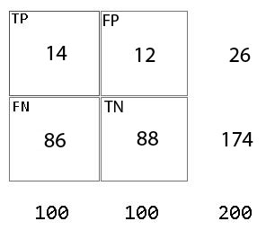
In an attempt to analyze some data as well as performance of my classifier and implementation on solar cavity detection I decided it would be beneficial to see the data in terms of individual quadrant performance. Below is the confusion matrix for the outcomes of the Quadrant III, based on 100 q3 (quadrant 3) positive images and 100 q3 (quadrant 3) negative images.
This matrix shows the outcomes from loading the classifier in raw form; without taking into consideration eliminating criteria such as proximity to disk, intensity, or template matching probability percentage just so I can show the significance of the elimination implementation. So to be clear, of the 100 positives for example I based the True Positive value on whether it correctly identified the solar cavity in that quadrant regardless of other detections it identified. So in keeping it essentially “black and white” or “Yes, it detected the cavity or No, it did not”.
Finally here is the confusion matrix, for the outcomes based on loading the classifier and then performing elimination criteria on the detected regions of interest. The classifier could sometimes return overlapping regions of interest. In terms of solar cavities I eliminate this as being applicable because I do not and have not really seen any solar cavities that are in that close of proximity that they would begin to overlap. So due to that the removal of overlapping regions of interest seems appropriate. I also set a range of values that when in gray scale it was a range of mid values and if the region of interest did not include some darker gray levels then the region is not considered a region of interest.
If the region of interest is not in close proximity to the disks edge (suns edge) then this can be eliminated as a region of interest since all solar cavities are close in proximity to the edge. Once the region has passed all the criteria above then we have our set of templates for each quadrant, that was designated as good samples of cavities within each quadrant. So a template matcher implementation is run on the region to further determine if it should be kept as a region of interest of discarded.
Tags: testing outcomes, thesis, trials
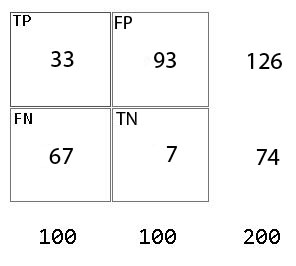
In an attempt to analyze some data as well as performance of my classifier and implementation on solar cavity detection I decided it would be beneficial to see the data in terms of individual quadrant performance. Below is the confusion matrix for the outcomes of the Quadrant II, based on 100 q2 (quadrant 2) positive images and 100 q2 (quadrant 2) negative images.
This matrix shows the outcomes from loading the classifier in raw form; without taking into consideration eliminating criteria such as proximity to disk, intensity, or template matching probability percentage just so I can show the significance of the elimination implementation. So to be clear, of the 100 positives for example I based the True Positive value on whether it correctly identified the solar cavity in that quadrant regardless of other detections it identified. So in keeping it essentially “black and white” or “Yes, it detected the cavity or No, it did not”.
Finally here is the confusion matrix, for the outcomes based on loading the classifier and then performing elimination criteria on the detected regions of interest. The classifier could sometimes return overlapping regions of interest. In terms of solar cavities I eliminate this as being applicable because I do not and have not really seen any solar cavities that are in that close of proximity that they would begin to overlap. So due to that the removal of overlapping regions of interest seems appropriate. I also set a range of values that when in gray scale it was a range of mid values and if the region of interest did not include some darker gray levels then the region is not considered a region of interest.
If the region of interest is not in close proximity to the disks edge (suns edge) then this can be eliminated as a region of interest since all solar cavities are close in proximity to the edge. Once the region has passed all the criteria above then we have our set of templates for each quadrant, that was designated as good samples of cavities within each quadrant. So a template matcher implementation is run on the region to further determine if it should be kept as a region of interest of discarded.
Tags: testing outcomes, thesis, trials
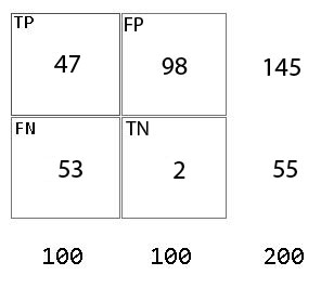
In an attempt to analyze some data as well as performance of my classifier and implementation on solar cavity detection I decided it would be beneficial to see the data in terms of individual quadrant performance. Below is the confusion matrix for the outcomes of the Quadrant I, based on 100 q1 (quadrant 1) positive images and 100 q1 (quadrant 1) negative images.
This matrix shows the outcomes from loading the classifier in raw form; without taking into consideration eliminating criteria such as proximity to disk, intensity, or template matching probability percentage just so I can show the significance of the elimination implementation. So to be clear, of the 100 positives for example I based the True Positive value on whether it correctly identified the solar cavity in that quadrant regardless of other detections it identified. So in keeping it essentially “black and white” or “Yes, it detected the cavity or No, it did not”.
Finally here is the confusion matrix, for the outcomes based on loading the classifier and then performing elimination criteria on the detected regions of interest. The classifier could sometimes return overlapping regions of interest. In terms of solar cavities I eliminate this as being applicable because I do not and have not really seen any solar cavities that are in that close of proximity that they would begin to overlap. So due to that the removal of overlapping regions of interest seems appropriate. I also set a range of values that when in gray scale it was a range of mid values and if the region of interest did not include some darker gray levels then the region is not considered a region of interest.
If the region of interest is not in close proximity to the disks edge (suns edge) then this can be eliminated as a region of interest since all solar cavities are close in proximity to the edge. Once the region has passed all the criteria above then we have our set of templates for each quadrant, that was designated as good samples of cavities within each quadrant. So a template matcher implementation is run on the region to further determine if it should be kept as a region of interest of discarded.
Tags: testing outcomes, thesis, trials
OpenCV has functionality built in for template matching. The template matching implementation is basically matching a subimage against a main image by sliding it across the entire image using one of the matching methods, in my implementations I used the normalized square difference matching method.
Below is a summarized excerpt for template matching within Quadrant 1.
const char* templateFilename = "F:\\Thesis_Research\\AutomatedDetector\\Test_Sets\\Quadrant_Images\\q1_faint.jpg";

// load template image
tpl = cvLoadImage( templateFilename, CV_LOAD_IMAGE_COLOR );
// Check if the template file loaded
if( tpl == 0 )
{
     fprintf( stderr, "Cannot load template file %s!\n", templateFilename  );
}

//Search quadrant 1
SearchQuadrant(1, img->width/2, 0, img->width/2, img->height/2);

CvRect region;
region = cvRect(img->width/2, 0, img->width/2, img->height/2);

//Get the width and height for the result image
width  = region.width  - tpl->width  + 1;
height = region.height - tpl->height + 1;

//Create a new image for comparison result
res = cvCreateImage( cvSize( width, height ), IPL_DEPTH_32F, 1 );

//Check if the result image was actually created
if( res == 0 )
{
     fprintf( stderr, "Cannot create new image for comparison result!\n" );
}

//Perform template matching
cvMatchTemplate( m_quadrant1Image, tpl, res, CV_TM_SQDIFF_NORMED );
The resultant image obtained is a single-channel byte of floating point image. Next, iteration through the image array to get the lowest threshold value. For cvMatchTemplate, a perfect match will be 0 and a bad match will be large. But there must be a defined line between the non perfect matches and non matches. I set my threshold to 0.05, and I take the lowest point beneath that threshold.
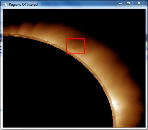
In running template matcher on positive images, for example the below image the lowest threshold was about 0.00621
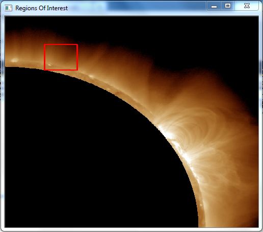
Below is the template matcher run on a negative image in order to determine a minimum threshold value of non cavity matches. But the negative image still returned a low value comparable to that of a positive detection of 0.00600 even though this was a negative image.
Tags: image processing, opencv, solar cavity
Below are examples of the haar-like feature sets that are used in training. It displays what features are used based on the “mode” option used as well as the string representation that will be used in each of the AdaBoostCARTHaarClassifier.txt files created for each stage on the classifier.
if(mode == BASIC || CORE || ALL)
haar_x2 haar_y2

haar_x3 haar_y3

haar_x2_y2
if(mode != BASIC)
haar_x4 haar_y4

haar_point
if(mode == ALL)
tilted_haar_x2 tilted_haar_y2

tilted_haar_x3 tilted_haar_y3

tilted_haar_x4 tilted_haar_y4

tilted_haar_point
One thing to notice is that tilted_haar_point feature is actually commented out in the cvhaartraining.cpp source code. So if that is a feature you would like to use it will need to be uncommented and recompiled for an new executable that will now include that feature.
Tags: haar training, opencv
Training Options Used –
-npos 1134
-nneg 625
-nstages 20
-mode ALL
The number of positive images used to train this classifier was 1134, the number of negative images used was 625 and specified that the number of stages the trainer should try to complete is 20. Used the mode ALL switch, which not only includes the basic haar like features but an extended set of features, here is a link to the feature sets Haar-like features. During the training phase of this cascade it finished in stage 20, which created 139 total weak classifiers. In this stage it reached the desired minimum false alarm rate, or else the false alarm rate will be too high for real world use.
NEG: 148 9.77509e-005
Used the OpenCV version of the haartraining.
opencv_haartraining.exe -data "F:\Thesis_Research\HaarClassifier\haarcascade15" -vec "F:\Thesis_Research\Test_Sets\Positive_Solar_Cavities\positivesoutput.vec" -bg "F:\Thesis_Research\Test_Sets\Negative_Solar_Cavities\negatives.txt" -npos 1134 -nneg 625 -nstages 20 -mode ALL
Hit rate ≈ 57.1%
Tags: testing outcomes, trials
