Once you have a *.xml file that you created from training the classifier then you can test the performance of that classifier cascade against your prositive test or you could create a validation test set to test performance against. OpenCV comes with a built in performance utility
C:\OpenCV2.2\bin>opencv_performance.exe -data "C:\My Documents\HaarClassifier\haarcascade\haarcascade.xml" -info "C:\My Documents\Positive Test Set\positivesoutput.txt"
Explanation of the code above:
opencv_performance.exe is a utility distributed with the OpenCV library. This is usually contained int the “bin” folder in the directory you installed OpenCV.
ex. C:\OpenCV2.2\bin
Below are the options available for this utility as well as what the defaults are.
C:\OpenCV2.2\bin>opencv_performance.exe
Usage: opencv_performance.exe
  -data <classifier_directory_name>
  -info <collection_file_name>
  [-maxSizeDiff <max_size_difference = 1.500000>]
  [-maxPosDiff <max_position_difference = 0.300000>]
  [-sf <scale_factor = 1.200000>]
  [-ni]
  [-nos <number_of_stages = -1>]
  [-rs <roc_size = 40>]
  [-w <sample_width = 24>]
  [-h <sample_height = 24>]
-ni – If specified it will not output the resultant image files with detections. If NOT specified it WILL create a new image for every image it opens and it will save it as det-[image filename] and it will contain boxes around the positive detections.
A small excerpt from the performance output:
+================================+======+======+======+
|            File Name           | Hits |Missed| False|
+================================+======+======+======+
|   20100627_001220_1024_0193.jpg|     0|     1|    19|
+--------------------------------+------+------+------+
|   20100627_002044_1024_0193.jpg|     1|     0|    16|
+--------------------------------+------+------+------+
|   20100627_004432_1024_0193.jpg|     1|     0|    17|
+--------------------------------+------+------+------+
|   20100627_005956_1024_0193.jpg|     1|     0|    20|
+--------------------------------+------+------+------+
|   20100627_010132_1024_0193.jpg|     1|     0|    16|
+--------------------------------+------+------+------+
|   20100627_011308_1024_0193.jpg|     0|     1|    22|
+--------------------------------+------+------+------+
|   20100627_014044_1024_0193.jpg|     1|     0|    21|
+--------------------------------+------+------+------+
|   20100627_015444_1024_0193.jpg|     1|     0|    18|
+--------------------------------+------+------+------+
|   20100627_015956_1024_0193.jpg|     1|     0|    17|
+--------------------------------+------+------+------+
|   20100627_021220_1024_0193.jpg|     1|     0|    18|
+--------------------------------+------+------+------+
|   20100627_021932_1024_0193.jpg|     1|     0|    18|
+--------------------------------+------+------+------+
...
...
+--------------------------------+------+------+------+
|                           Total|  1009|   352| 10532|
+================================+======+======+======+
Number of stages: 18
Number of weak classifiers: 98
Total time: 9.734000
18
        41      93      0.431579        0.978947
        41      93      0.431579        0.978947
        41      93      0.431579        0.978947
        39      38      0.410526        0.400000
        38      28      0.400000        0.294737
        38      22      0.400000        0.231579
        34      16      0.357895        0.168421
        ...
        ...
For metrics and data analysis this can be very helpful as it will not only give you the performance but also the number of stages the classifier used and the number of weak classifiers used in this cascade.
This is an easy way of seeing your classifiers performance right away, and based on the results you can tell whether your classifier is really performing poorly (No Hits and/or Alot of False Hits). If this is the case it would be best to start the process over and maybe get more positive and negative training samples.
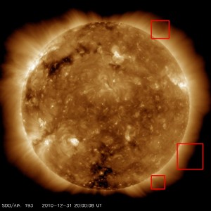
Example of image file created when I did not use the -ni option. (It will mark all the objects it calculates as”positive” areas, so hits and false hits will show up).
Tags: command prompt, Haar Classifier, haar training, opencv, thesis
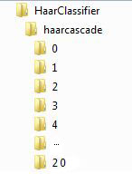
Once your training is done there will be a number of directories created in your haarcascade location you specified when your training first began. The directories will be labelled from 0…N where N is the total number of stages the trainer completed. In each directory there will be one AdaBoostCARTHaarClassisifer.txt file and each of the files contains information about that particular one stage of classifiers. In other words, a cascaded boost Haar classifier is composed of N stages of classifiers.
Below is an example of the contents of the AdaBoostCARTHaarClassisifer.txt file that is created in every stage of the training.
A excerpt from the stage 0 classifier output:
3
1
2
0 6 18 7 0 -1
9 6 9 7 0 2
haar_x2
-7.839686e-002 0 -1
6.697344e-001 -6.912314e-001
1
2
9 0 7 22 0 -1
9 11 7 11 0 2
haar_y2
2.000804e-001 0 -1
-6.013643e-001 6.833895e-001
1
2
3 0 9 2 0 -1
3 1 9 1 0 2
haar_y2
1.305457e-004 0 -1
-9.137786e-001 4.921354e-001
-8.454085e-001

-1
-1
Line 1: is the number of (weak) classifiers in this current stage that will ultimately be a part of the final strong classifier.
Line 2: is the number of nodes in this decision tree. Since each of classifier is viewed as a single node decision tree, all of my weak classifiers are all composed of only 1 node.
Line 3: is the number of rectangles involved in computing a Haar-like feature.
Line 4: 6 integers representing the parameters of the 1st rectangle.
1st value – x-coordinate of the top-left corner (r.x)
2nd value – y-coordinate of the top-left corner (r.y)
3rd value – width of rectangle (r.width)
4th value – height of rectangle (r.height)
5th value – band of the rectangle
6th value – weight of the rectangle
Line 5: 6 integers representing the parameters of the 2nd rectangle
(See Line 4: for definitions)
Line 6: A string displaying the haar feature type used
Line 7: 3 integers representing branches
1st value – Branches threshold if the value is
2nd value – Index of left branch
3rd value – Index of right branch
Line 8: Output value corresponding to the leaf
Tags: Haar Classifier, haar training, opencv
When going through the training stages you might find that your training has come to a halt where its progress isn’t getting any further and or it has exited out improperly. If this happens you can still turn the stages it did successfully complete into a Classifier Cascade XML.
OpenCV comes with a built in cascade conversion utility that seems to work pretty well.
convert_cascade.exe --size="24x24" "C:\MyDocuments\HaarClassifier\haarcascade" haarcascade.xml
Explanation of the code above:
convert_cascade.exe is a utility distributed with the OpenCV library. This is usually contained int the “samples\c” folder in the directory you installed OpenCV.
ex. C:\OpenCV2.2\samples\c
Below are the options available for this utility.
Usage:
convert_cascade.exe --size="<width>x<height>" <input_cascade_path> <output_cascade_filename>
–size – Is the size dimensions you have specified for your positive detections. In my case –size=”24×24″
input_cascade_path – This is the directory that holds your incomplete haarcascade. From the Training post its the -data “C:\My Documents\HaarClassifier\haarcascade” location
output_cascade_filename – Specify a output name for your xml file. haarcascade.xml
Tags: Haar Classifier, haar training, opencv
Once you have a *.vec file that you created from your positive images you are ready to train your classifier. OpenCV comes with a built in training utility
opencv_haartraining.exe -data "C:\My Documents\HaarClassifier\haarcascade" -vec "C:\My Documents\Positive Test Set\positives.vec" -bg "C:\My Documents\Negative Test Set\negatives.txt" -npos 1134 -nneg 625 -nstages 20
Explanation of the code above:
opencv_haartraining.exe is a utility distributed with the OpenCV library. This is usually contained int the “bin” folder in the directory you installed OpenCV.
ex. C:\OpenCV2.2\bin
Below are the options available for this utility as well as what the defaults are.
Usage: opencv_haartraining.exe
  -data <dir_name>
  -vec <vec_file_name>
  -bg <background_file_name>
  [-bg-vecfile]
  [-npos <number_of_positive_samples = 2000>]
  [-nneg <number_of_negative_samples = 2000>]
  [-nstages <number_of_stages = 14>]
  [-nsplits <number_of_splits = 1>]
  [-mem <memory_in_MB = 200>]
  [-sym (default)] [-nonsym]
  [-minhitrate <min_hit_rate = 0.995000>]
  [-maxfalsealarm <max_false_alarm_rate = 0.500000>]
  [-weighttrimming <weight_trimming = 0.950000>]
  [-eqw]
  [-mode <BASIC (default) | CORE | ALL>]
  [-w <sample_width = 24>]
  [-h <sample_height = 24>]
  [-bt <DAB | RAB | LB | GAB (default)>]
  [-err <misclass (default) | gini | entropy>]
  [-maxtreesplits <max_number_of_splits_in_tree_cascade = 0>]
  [-minpos <min_number_of_positive_samples_per_cluster = 500>]
From my example of the usage I just kept everything as the default, aside from my number of positives and negatives and how many stages I wanted, typically the larger the number of stages you will achieve a better false alarm rates but it will take more time generating your final cascade. It does not make sense to increase the number of stages when you have a small number of positive and negative samples. The system will attempt to build a classifier with the desired hit rate, then it will calculate its false alarm rate and if the false alarm rate is higher than the max false alarm rate it will reject the classifier and will build the next classifier.
A small excerpt from the training output:
Tree Classifier
Stage
+---+
|  0|
+---+

   0

Parent node: 0

*** 1 cluster ***
POS: 282 283 0.996466
NEG: 155 0.54007
BACKGROUND PROCESSING TIME: 0.03
Precalculation time: 0.07
+----+----+-+---------+---------+---------+---------+
|  N |%SMP|F|  ST.THR |    HR   |    FA   | EXP. ERR|
+----+----+-+---------+---------+---------+---------+
|   1|100%|-|-0.874803| 1.000000| 1.000000| 0.139588|
+----+----+-+---------+---------+---------+---------+
|   2|100%|+|-0.722001| 1.000000| 0.774194| 0.105263|
+----+----+-+---------+---------+---------+---------+
|   3| 91%|-|-0.179203| 0.996454| 0.303226| 0.155606|
+----+----+-+---------+---------+---------+---------+
Stage training time: 59.56
Number of used features: 3

Parent node: 0
Chosen number of splits: 0

Total number of splits: 0
N – Current feature for this cascade
%SMP – Percentage of samples used
F – ‘+’ if symmetry is specified
ST.THR – Stage Threshold
HR – Hit Rate based on the ST.THR (hitrate/numpos)
FA – False Alarm based on ST.THR (falsealarm/numneg)
EXP.ERR – Strong Classification of Adaboost Algorithm, based on threshold
One thing observed is that while in the training phase you will go to some forums where the trainer has been running for more than 4 days and some people saying that it took them a number of weeks, well sometimes the trainer will get into an infinite loop state and as a user you will never know that its really not running. SO, after finding this out when I began wondering why my trainer was still on the same training stage for 4 days. So for example if you specify 20 stages and say at stage 17 your NEG: 365 2.52601e-006 rate gets about to or below the rate it will just sit there, and you must exit out. After finding this out I went into the source code and made some modifications so it will not get into this state as well as tailored it to my wants and needs.
After the training completes successfully it will generate an XML that is your combined cascade of all the weak classifiers.
A small excerpt from the xml output:
<?xml version="1.0"?>
<opencv_storage>
<haarcascade8 type_id="opencv-haar-classifier">
  <size>
    24 24</size>
  <stages>
    <_>
      <!-- stage 0 -->
      <trees>
        <_>
          <!-- tree 0 -->
          <_>
            <!-- root node -->
            <feature>
              <rects>
                <_>
                  0 6 18 7 -1.</_>
                <_>
                  9 6 9 7 2.</_></rects>
              <tilted>0</tilted></feature>
            <threshold>-7.8396856784820557e-002</threshold>
            <left_val>6.6973441839218140e-001</left_val>
            <right_val>-6.9123142957687378e-001</right_val></_></_>
        <_>
Tags: Haar Classifier, haar training, opencv
Once you have a file that lists your positive images with the corresponding positive locations within each image you can then create a training sample based off of this file that will then create a vector of samples and translations to be used to train your classifier.
opencv_createsamples.exe -info "C:\My Documents\Positive Test Set\positives.txt" -vec "C:\My Documents\Positive Test Set\positives.vec"
Explanation of the code above:
opencv_createsamples.exe is a utility distributed with the OpenCV library. This is usually contained int the “bin” folder in the directory you installed OpenCV.
ex. C:\OpenCV2.2\bin
Below are the options available for this utility as well as what the defaults are.
Usage: opencv_createsamples.exe
  [-info <collection_file_name>]
  [-img <image_file_name>]
  [-vec <vec_file_name>]
  [-bg <background_file_name>]
  [-num <number_of_samples = 1000>]
  [-bgcolor <background_color = 0>]
  [-inv] [-randinv] [-bgthresh <background_color_threshold = 80>]
  [-maxidev <max_intensity_deviation = 40>]
  [-maxxangle <max_x_rotation_angle = 1.100000>]
  [-maxyangle <max_y_rotation_angle = 1.100000>]
  [-maxzangle <max_z_rotation_angle = 0.500000>]
  [-show [<scale = 4.000000>]]
  [-w <sample_width = 24>]
  [-h <sample_height = 24>]
From my example of the usage I just kept everything as the default. I did create a number of vector files by specifying different options and values, but of those I found my classifier results to be undesired. So I need to come up with better values for these options, but for the time being since my time for implementation is short. I might come back to this and fine tune when I have the time.
The vector file created will contain information non readable to you, but its your way of knowing it worked.
A small excerpt from the file:
 è D D C @ < ; < ; 7 6 5 3 3 5 2 / - , + * ( ' & $ D D C @ < ;
< ; 7 7 5 3 3 5 3 / - , + * ( ' & $ D D C @ =
; < ; 7 7 5 3 3 5 3 / - , , * ( ' & % E E D A > < = ; 9 8 5 4 4 5 2 /
 i e a ] Z X W W V U W Y W U R P N O „ ~ | z u o j e d _ \ Z Z
Tags: create samples, Haar Classifier
How do we tell our program what we want to look for?
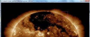
I created a directory full of positive images (images that contain the object(s) that I want to identify) and I created a directory full of images that I know do not contain any of the objects that I want to identify. My positive image count was about 1134 and my negative image count was about 625. In all other posts and papers I have read it seems that the more images you have the better coverage you get on the differences in such things as scale, orientation, distortion.
But you also have to take into account if you have over 1000 images you will have to sit through and mark every one of those images with boxes identifying the objects and positions in each image and this can be really time consuming. You may ask surely there is a way of automating this? But if this was automated then you would already have the exact thing you are trying to make in the first place… 🙂

So sit back and get comfortable because you could be there for awhile. So is it better to spend the time up front and the program execute and identify fast, or have a program take forever identifying objects at run time? Guess its all about what you want/need from your implementation.
To run the ObjectMarker executable
ObjectMarker.exe <outputfile> <directory of jpg images to mark>
Once you are done marking all the images you should have a new output file that its contents should look something like this
filename <no. of objects marked in the image> <top left corner x-coordinate> <top left corner y-coordinate> <width of rectangle> <height of rectangle>
20100627_001220_1024_0193.jpg 1 705 127 22 6

20100627_002044_1024_0193.jpg 1 705 127 58 62

20100627_004432_1024_0193.jpg 1 715 135 48 54

20100627_005956_1024_0193.jpg 1 715 135 46 54

20100627_010132_1024_0193.jpg 1 712 132 49 57

20100627_011308_1024_0193.jpg 1 721 144 37 40

20100627_014044_1024_0193.jpg 1 720 142 40 49

20100627_015444_1024_0193.jpg 1 705 137 63 59

20100627_015956_1024_0193.jpg 1 707 136 66 60

20100627_021220_1024_0193.jpg 1 711 137 58 54

20100627_021932_1024_0193.jpg 1 704 137 66 56

20100627_025432_1024_0193.jpg 1 699 136 69 55

20100627_031156_1024_0193.jpg 1 695 141 77 52

20100627_032208_1024_0193.jpg 1 699 137 73 53

20100901_010108_1024_0193.jpg 2 761 799 93 94 803 216 34 44
Tags: Haar Classifier
This is specifically for Windows using the command prompt. When doing image processing and classifcations you’ll find yourself with directories full of images. And in some cases if you choose to use a learner you’ll have to load each image in your postives and/or negatives directory. So you can just list your image names in a file and just load that text file, and in OpenCV if you choose to use a HaarClassifier this is needed.
cd "C:\My Documents\Positive Test Set"

dir /B "*.jpg" > positives.txt
Explanation of the code above:
cd <directory with images>
cd – Change directories, you will want to be in the directory that you want to list the files from.
dir /B "*.jpg" > <outputfile>
dir – Displays all files in directory.
/B – Means bare format (no heading information or summary) We don’t care about size, date, time etc… we only want the filename.
“*.jpg” – In this example I only want jpg files.
> – This is a redirection operator ‘>’. Really what its saying is instead of printing the results in the command prompt window send it to a file.
The output files contents will look like this
20110507_002544_1024_0193.jpg

20110507_004120_1024_0193.jpg

20110507_005632_1024_0193.jpg

20110507_011120_1024_0193.jpg

20110507_012544_1024_0193.jpg

20110507_014232_1024_0193.jpg

20110507_015956_1024_0193.jpg

20110507_021456_1024_0193.jpg

20110507_022844_1024_0193.jpg

20110507_024144_1024_0193.jpg
Tags: command prompt
Machine Learning is a rapidly growing Haar Classifier is a supervised classifier, it has mainly been used for facial detection but it can also be trained to detect other objects. Computer vision is such a growing field that there are so many resources available for your own personal use. OpenCV provides a lot of functionality for machine learning techniques and the Haar Classifier is one of them. I thought this could potentially be good for use in recognition of solar cavities, because of its robustness, ease of use, built in basic OpenCV functionality and I found that it runs a lot faster than other techniques I tried to implement.
The Haar Feature supported by OpenCV is an object detector initially proposed by Paul Viola and Michael Jones in Rapid Object Detection using a Boosted Cascade of Simple Features
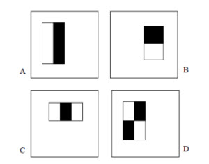
Example rectangle features shown relative to the enclosing detection window. The sum of the pixels which lie within the white rectangles are subtracted from the sum of pixels in the black rectangles. Two-rectangle features are shown in (A) and (B). Figure (C) shows a three-rectangle feature, and (D) a four-rectangle feature.
This technique harbors on the concept of using features rather than pixels directly. Which can then be easier to process and gain domain knowledge from correlating feature sets. It has also proven to be exceptionally faster than that of pixel relation systems
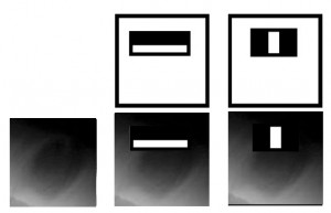
The first and second features selected by AdaBoost.
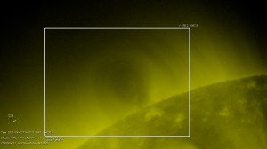
The two features are shown in the top row and then overlayed on a typical training cavity in the bottom row. The first feature measures the difference in intensity between the region of the top portion with the region right below. The feature capitalizes on the observation that the top region is often darker than lower parts of the cavity (a gradient). The second feature compares the intensities in the middle regions to the intensity across the outer edges of the cavity.
A Haar Classifier is really a cascade of boosted classifiers working with haar-like features. Haar-like features are specific adjacent rectangular regions at a specific location in a window (as shown in the first image above). The difference is then used to categorize subsections of an image and separates the non-objects from objects. Due to this distinction it is more of a weak learner, where you must use a large number positives to get as many Haar-like features as possible to accurately describe an object with some type of correlation and accuracy. So with all of these essentially weak classifiers we combine them into our classifier cascade to hopefully form a strong learner, by way of boosting.
Boosting is the concept of creating a set of weak learners and combining them to make a single strong learner. In the implementation of detecting solar cavities I used the AdaBoosting algorithm (aka Adaptive Boosting). This algorithm was initially proposed by Yoav Freund and Robert Schapire in A Decision-Theoretic Generalization of on-Line Learning and an Application to Boosting. It is used to improve a learning algorithms performance, by calling weak classifiers repeatedly and updating weights.
OpenCV currently supports multiple variations of AdaBoost including Discrete Adaboost, Real Adaboost, Gentle Adaboost and Logitboost.
Tags: Haar Classifier, thesis
OpenCV is an image processing library that I use in conjunction with C++ in Visual Studio. This library has proven to be very useful so far. I have experienced a number of crashes, as well as using some of their supplied binaries. Some of these I was able to get around by actually loading the source code and compiling it myself with debug information so I could further see what the problem was. Since I have done this my understanding of OpenCV has gotten better as well as developing thoughts on how to be a better programmer and include status message or more descriptive error parsing…. but we can’t expect every developer to be so forth coming. That being said, no code is error free sometimes as a developer you will have to dig further into the libraries and binaries supplied to get it working for what you want/need.
OpenCV can be downloaded here… Read the rest of this entry »
Tags: image processing, opencv
Solar Cavities are said (in theory) to be precursors to CMEs (Coronal Mass Ejections). These prominences are therefor clues to the state of the corona prior to emitting a CME, which in turn could be the signature of stored magnetic energy that is then capable of creating and driving the CME.
Tags: solar cavity, thesis
